Use CNN Architecture To Classify Handwritten Digits

29 Mar 2020 in Kaggle Competitions

This is a digit recognizer that is used to classify handwritten digits (the classic MNIST dataset). It uses machine learning to train a small convolutional neural network to achieve the goal. I utilized techniques such as dataset augmentation and early stopping in training and achieved 99.4% accuracy on the testing data.

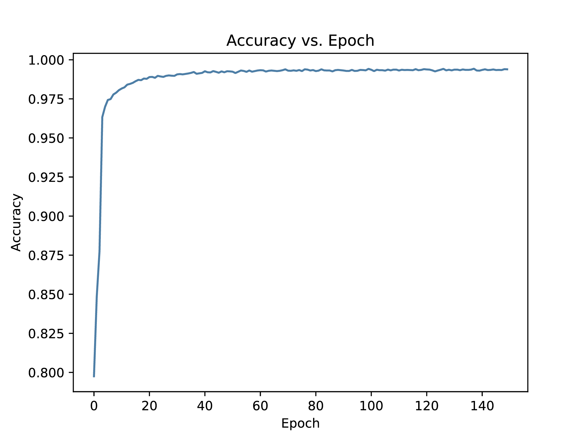
This is a digit recognizer that is used to classify handwritten digits (the classic MNIST dataset). It uses pytorch machine learning framework to train a small convolutional neural network to achieve the goal. I utilized techniques such as dataset augmentation and early stopping in training and achieved 99.4% accuracy on the testing data.

This project is developed for the Kaggle Digit Recognizer competition and data is provided by Kaggle. My source code and model can be found on by github.

Part 1 - Data Preperation

Kaggle provided a dataset of 42,000 images with labels and 28,000 images without labels for testing. Those data are loaded using the pandas module. The entire dataset is divided into a training set and a validation set. Although this will reduce the number of images for training, it can help to understand the model’s performance during training, which can be used to estimate the actual testing accuracy (out sample error).

import numpy as np
import pandas as pd
from sklearn.model_selection import train_test_split

raw_data = pd.read_csv('train.csv', dtype=np.float32)

labels = dataset.label.values
features = dataset.loc[:, dataset.columns != 'label'].values / 255.
data_train, data_val, labels_train, labels_val = train_test_split(features, labels, test_size=0.25)

print(data_train.shape, labels_train.shape)     # output: (31500, 784) (31500,)
print(data_val.shape, labels_val.shape)         # output: (10500, 784) (10500,)

Since we reduced the size of the training set, tricks like dataset augmentation can be used. Giving the nature of handwritten digits, an image of digit shifted by a pixel in any direction should not change the number recognized. This not only increases the number of images available for training but also introduces location invariance to the model (able to recognize digit regardless where that digit appears in the image).

from scipy.ndimage import shift

def shift_left(img):
    return shift(img.reshape(28, 28), [0, -1])

def shift_right(img):
    return shift(img.reshape(28, 28), [0, 1])

def shift_up(img):
    return shift(img.reshape(28, 28), [-1, 0])

def shift_down(img):
    return shift(img.reshape(28, 28), [1, 0])

aug_data = data_train.reshape(-1, 28, 28)   # augmented data for training
aug_data = np.r_[aug_data, np.apply_along_axis(shift_left, 1, data_train)]
aug_data = np.r_[aug_data, np.apply_along_axis(shift_right, 1, data_train)]
aug_data = np.r_[aug_data, np.apply_along_axis(shift_up, 1, data_train)]
aug_data = np.r_[aug_data, np.apply_along_axis(shift_down, 1, data_train)]
aug_label = np.r_[labels_train, labels_train, labels_train, labels_train, labels_train]

print(aug_data.shape, aug_label.shape)     # output: (157500, 28, 28) (157500,)

Another set of transformations we can apply is rotation. This is slightly tricky because it can change the class if an image is rotated significantly. For example, an image of 6 rotated by 180 degrees will become 9, which is a different class. In the current project, a rotation of $\pm10\degree$ is applied.

from scipy.ndimage import rotate

def clockwise_rotate(img):
    return rotate(img.reshape(28, 28), -10, reshape=False)

def counterclockwise_rotate(img):
    return rotate(img.reshape(28, 28), 10, reshape=False)

aug_data = np.r_[aug_data, np.apply_along_axis(clockwise_rotate, 1, data_train)]
aug_data = np.r_[aug_data, np.apply_along_axis(counterclockwise_rotate, 1, data_train)]
aug_label = np.r_[aug_label, labels_train, labels_train]

print(aug_data.shape, aug_label.shape)     # output: (220500, 28, 28) (220500,)

Now all data are ready. Note that those transformations are not allied applied to the validation set since the goal of the validation set is to gain an unbiased estimation of the testing error. The next step is to load these data into torch tensor and prepare the dataset and loader.

import torch

data_train = torch.from_numpy(aug_data.reshape(-1, 1, 28, 28)).type(torch.cuda.FloatTensor)
labels_train = torch.from_numpy(aug_label.reshape(-1)).type(torch.cuda.LongTensor)
train = torch.utils.data.TensorDataset(data_train, labels_train)

data_val = torch.from_numpy(data_val.reshape(-1, 1, 28, 28)).type(torch.cuda.FloatTensor)
labels_val = torch.from_numpy(labels_val.reshape(-1)).type(torch.cuda.LongTensor)
val = torch.utils.data.TensorDataset(data_val, labels_val)

Part 2 - Neural Network Model

Fig. 1 - The architecture of a simple CNN used for this project.

The simple CNN architecture consists of 2 convolutional layers followed by 3 fully connected layers as shown in Fig. 1. Here is the detail of the neural network:

1. Convolution layer: 64 filters of size $5\times5$ with stride 1 and no padding. ReLU activation is applied to the output. The output shape is $(64, 24, 24)$.
2. Dropout layer: $p=0.5$.
3. Maxpool layer: size $2\times2$ with stride 2 and no padding. The output shape is $(64, 12, 12)$.
4. Convolution layer: 256 filters of size $3\times3$ with stride 1 and no padding. ReLU activation is applied to the output. The output shape is $(256, 10, 10)$.
5. Dropout layer: $p=0.5$.
6. Maxpool layer: size $2\times2$ with stride 2 and no padding. The output shape is $(256, 5, 5)$.
7. Fully connected layer: 256 neurons. ReLU activation is applied to the output. The output shape is $(256)$.
8. Dropout layer: $p=0.5$.
9. Fully connected layer: 64 neurons. ReLU activation is applied to the output. The output shape is $(64)$.
10. Dropout layer: $p=0.5$.
11. Fully connected layer: 10 neurons. Softmax activation is applied to the output. The output shape is $(10)$.

Here is the torch implementation for the network:

import torch.nn as nn

class DigitRecognizerNN(nn.Module):

    def __init__(self):
        super(DigitRecognizerNN, self).__init__()
        self.min_loss = 1e10        # used to early stopping - explained later
        self.max_state_dict = None  # used to early stopping - explained later

        self.conv1 = nn.Conv2d(in_channels=1, out_channels=64, kernel_size=5)
        self.relu1 = nn.ReLU()
        self.drop1 = nn.Dropout()
        self.pool1 = nn.MaxPool2d(kernel_size=2)
        self.conv2 = nn.Conv2d(in_channels=64, out_channels=256, kernel_size=3)
        self.relu2 = nn.ReLU()
        self.drop2 = nn.Dropout()
        self.pool2 = nn.MaxPool2d(kernel_size=2)

        self.fc1 = nn.Linear(256 * 5 * 5, 256)
        self.relu3 = nn.ReLU()
        self.drop3 = nn.Dropout()
        self.fc2 = nn.Linear(256, 64)
        self.relu4 = nn.ReLU()
        self.drop4 = nn.Dropout()
        self.fc3 = nn.Linear(64, 10)
        self.softmax = nn.Softmax(dim=1)

    def forward(self, x):
        x = self.drop1(self.relu1(self.conv1(x)))
        x = self.pool1(x)
        x = self.drop2(self.relu2(self.conv2(x)))
        x = self.pool2(x)

        x = x.view(x.size(0), -1)
        x = self.drop3(self.relu3(self.fc1(x)))
        x = self.drop4(self.relu4(self.fc2(x)))
        return self.softmax(self.fc3(x))

    def record_state(self, loss):
        # used to early stopping - explained later
        self.min_loss = loss
        self.max_state_dict = self.state_dict()

The selection of the number of kernels, the filter size, and other parameters are decided based on trial-and-error. This model is a bit of an overkill for a simple task like this. Feel free to play with my model architecture and aim for higher accuracy!

Part 3 - Training

There are few hyperparameters I set to train the model: batch size, learning rate, and the number of epochs. I have added the parameter for $L^2$ penalty but not used. I’ll explain all hyperparameter choices briefly. All of them are chosen based on trial-and-error; there is no perfect answer for these parameters.

BATCH_SIZE = 4096   # may need to be tuned based on the hardware
LEARNING_RATE = 0.0002
NUM_EPOCHS = 150
L2_PENALTY = 0

• Batch size: bigger the better (as long as the hardware can handle it)? I have an RTX 2080 Ti which allows large batch size. Large batch size does make a large gradient step which can add difficulties to the training process. I reduced the learning rate to a small number in order to compensate the large batch size.
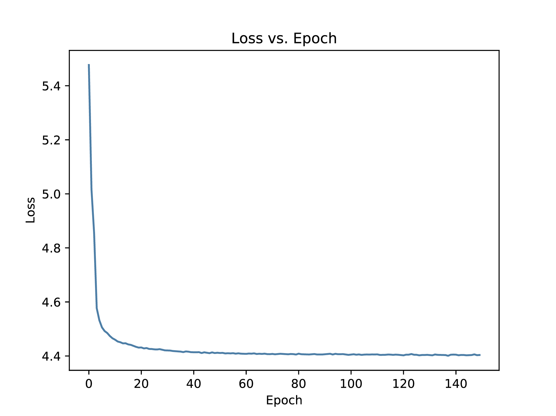
• Learning rate and optimizer: I am using Adam optimizer with default $\beta_1$ and $\beta_2$ which are the decay rate for moment estimation. Adam is an optimizer with an adaptive learning rate, which is a common choice for many problems. I’ve tried with a default learning rate of 0.001 but the validation loss fluctuates significantly between epochs, indicating there is overshoot in gradient steps. I ended up with a 0.0002 learning rate which takes a long time to train but has almost constant validation loss after 40-50 epochs.
• Number of epochs: Here I defined 1 epoch as one full pass through the entire dataset. However, there are multiple gradient steps (parameter updates) for one epoch. The training procedure is set up to return the set of parameters with the least validation error (early stopping) and there are aggressive dropouts in the model, so the harm from excessive training is limited except for wasting time. I am training for 150 epochs so that the model can explore fully near the local optimum. This is another overkill for training. For practical approaches, 10 epochs can achieve $0.980$ accuracy and 30 epochs can achieve $0.990$ accuracy. I used 150 and was able to achieve $0.995$ accuracy.
• $L^2$ penalty: I tried to add $L^2$ penalty to the loss function, however, I did not see any noticeable improvements. Theories have shown that the effect of $L^2$ penalty is mathematically equivalent to early stopping using quadratic approximation (see the deep learning book by Ian Goodfellow et. al for detail). Since I have implemented early stopping and experimental results from using norm penalties is not obvious, I have decided not to use it.
• Loss function: I picked cross-entropy loss for the problem. Again this is a common choice for a multi-class classification problem like MNIST. The log operation in the loss works well with the exponent in the softmax to avoid problems like diminishing/exploding gradient.

For every epoch, the model is evaluated using the validation set to obtain accuracy and loss value. Once the loss is lower than the history loss value, the parameter at the current stage is stored and will be used to evaluate the model later. An argument can be made that validation should be performed for every gradient update. It can guarantee we never miss a state of minimum loss but it adds significant overhead to training. For practical reasons, I have decided to validate every full pass after the training set instead of every batch.

Here is the code for training the model:

def validate_model(model, loss, val_loader):
    correct = 0
    total = 0
    total_loss = 0.0
    model.eval()
    for features, labels in val_loader:
        # Forward propagation
        outputs = model(features)
        compute_loss = loss(outputs, labels)

        # Get predictions from the maximum value
        predicted = torch.max(outputs.data, 1)[1]

        # Total number of labels
        total += len(labels)
        correct += (predicted == labels).sum()
        total_loss += compute_loss.data
    return total_loss, float(correct) / total

def train_model(model, optimizer, loss, train_loader, val_loader, num_epochs):
    history = {'loss': [], 'accu': []}

    for epoch in range(num_epochs):
        model.train()
        start_time = time.time()
        for features, labels in train_loader:
            optimizer.zero_grad()

            # Forward propagation
            outputs = model(features)

            # Calculate the loss for current epoch
            compute_loss = loss(outputs, labels)

            # Calculating gradients
            compute_loss.backward()

            # Update parameters
            optimizer.step()
        end_time = time.time()
        val_loss, val_accu = validate_model(model, loss, val_loader)
        history['loss'].append(val_loss)
        history['accu'].append(val_accu)

        if val_loss < model.min_loss:
            model.record_state(val_loss)

    return history

train_loader = torch.utils.data.DataLoader(train, batch_size=BATCH_SIZE, shuffle=True)
val_loader = torch.utils.data.DataLoader(val, batch_size=BATCH_SIZE, shuffle=True)

model = DigitRecognizerNN()
model.cuda()
loss = nn.CrossEntropyLoss()
optimizer = optim.Adam(model.parameters(), lr=LEARNING_RATE, weight_decay=L2_PENALTY)

# the training metadata is used for plotting
history = train_and_validate_model(model, optimizer, loss, train_loader, val_loader, NUM_EPOCHS, 1)

torch.save(model.max_state_dict, 'model.pt')

Here are the graph for loss and accuracy over epochs.

Fig. 2 - The validation loss of the model during training.

Fig. 1 - The validation accuracy of the model during training.

Part 4 - Testing

Testing is similar to the validation process for training with the testing data. The general steps are 1) load testing data and pre-trained model, 2) run the model on the testing data, and 3) save the output to csv file for submission.

def test_model(model, testing_data_loader):
    predictions = []
    model.eval()
    for feature in data_loader:
        # Forward propagation
        output = model(feature[0])
        predictions += (torch.max(output.data, 1)[1]).tolist()

    return predictions

dataset = pd.read_csv('sample_submission.csv', dtype=np.float32)
data_test = dataset.loc[:, dataset.columns != 'label'].values / 255.
data_test = torch.from_numpy(data_test.reshape(-1, 1, 28, 28)).type(torch.cuda.FloatTensor)

testing = torch.utils.data.TensorDataset(data_test)
testing_data_loader = torch.utils.data.DataLoader(testing, batch_size=BATCH_SIZE, shuffle=False)

model = DigitRecognizerNN()
model.cuda()
model.load_state_dict(torch.load('model/DigitRecognizer/model.pt'))
output = test_model(model, testing_data_loader)

dataset = dataset.assign(Label=output)
dataset.to_csv('submission.csv', index=False)

One thing to keep in mind is that make sure the testing data is not shuffled.

Part 5 - Future Work

As I said before, some hyperparameter settings for this is an overkill and can be tuned further. Few things potentially can make the model better:

1. Another form of transformation that can be added is zooming. Although all images come with a fixed resolution, the numbers in each image can have varying sizes. Zooming can also be a technique used for dataset augmentation.
2. Aggressive dropout is used on this “complex model” (complex in terms of the problem it is trying to solve). A simpler model with less aggressive dropout and appropriate regularization can have a similar result. 3, I used the validation set for validation purposes only, which is taking away data for training. A better practice would be using the validation data to determine hyperparameters and combine the validation set with training set to produce a model with a better fit.

There are more things can be added to solve this problem. Feel free to explore more possibilities!